fast-robots

Lab 2

For this lab, we started working with the IMU sensor and the RC car.

Setup

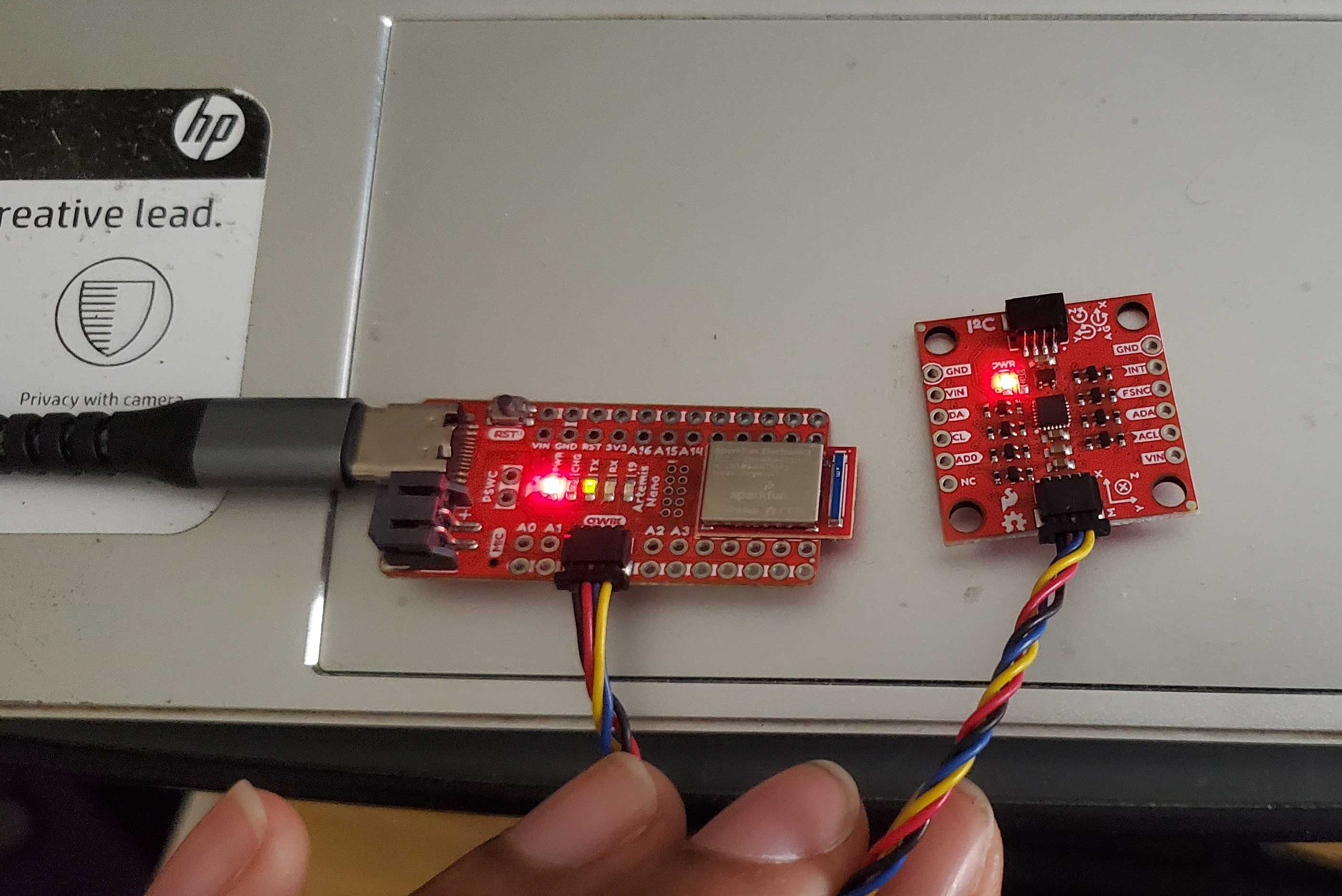
After installing the appropriate Arduino library for the IMU and connecting it to the Artemis Nano board using QWIIC connectors, I tested its functionality using the Example1_Basics file from the Arduino library. The AD0_VAL definition refers to the last bit of the address for the IMU for reading/writing data, so I left it at its default value of 1. I also added a simple flashing LED signal to indicate that the board is running for convenience of data measurement.

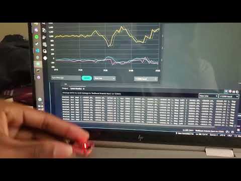
Here, program execution works as intended. I show gyroscope data by rotating the IMU across all axes, then I show accelerometer data using the serial plotter, with acceleration along the X, Y, and Z axes plotted on the pink, blue, and yellow lines, respectively.

Accelerometer

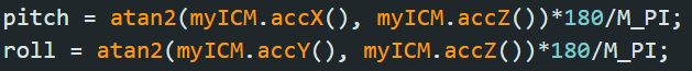
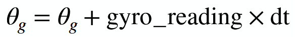
Working with the accelerometer now, my first task was to use the sensor data to find pitch and roll using the equations from class. Below I reproduce those equations:

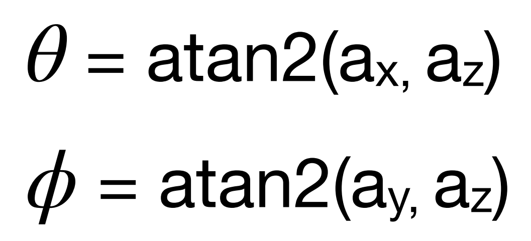
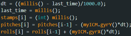
Followed by my implementation in Arduino, maintained as global variables:

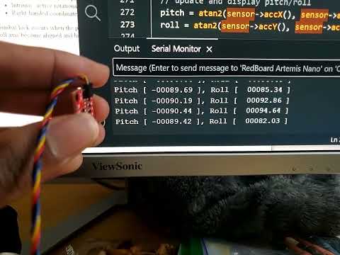
And here is a short clip of my output with pitch of -90 degrees and roll of +90 degrees:

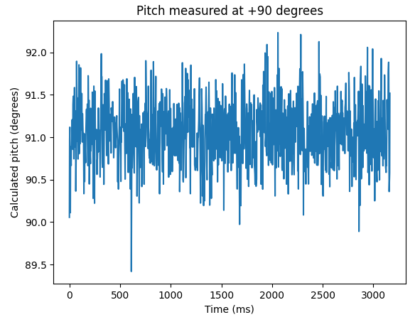
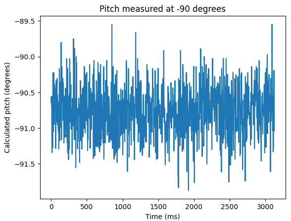
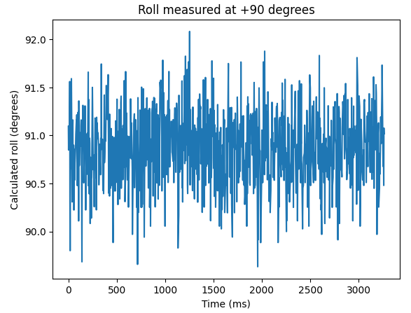
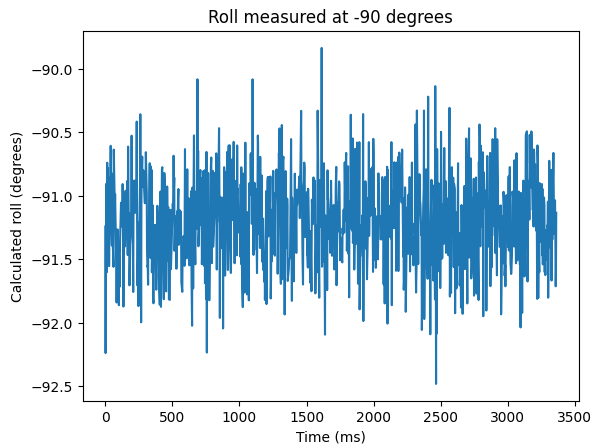
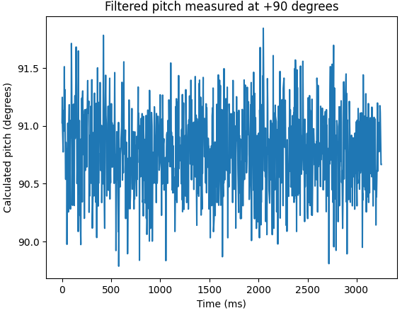
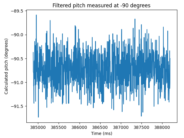
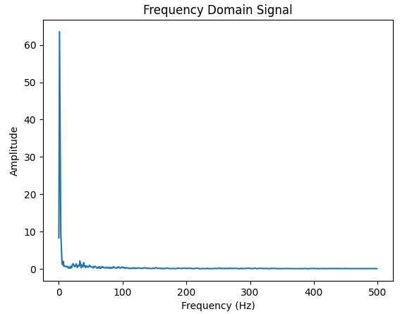
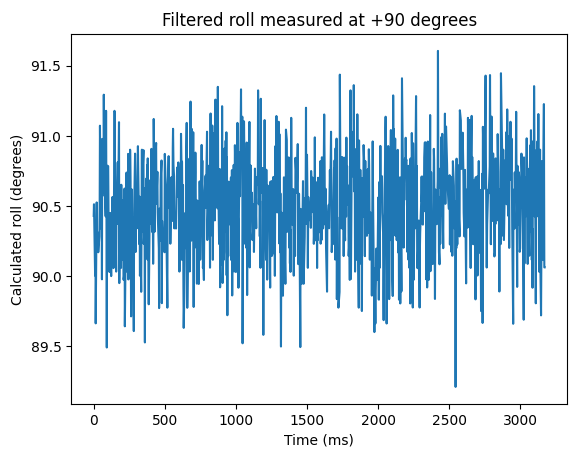
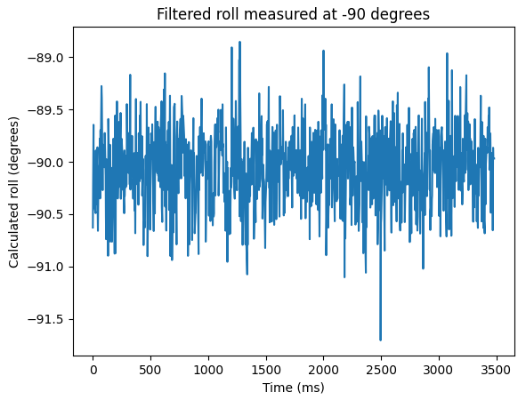
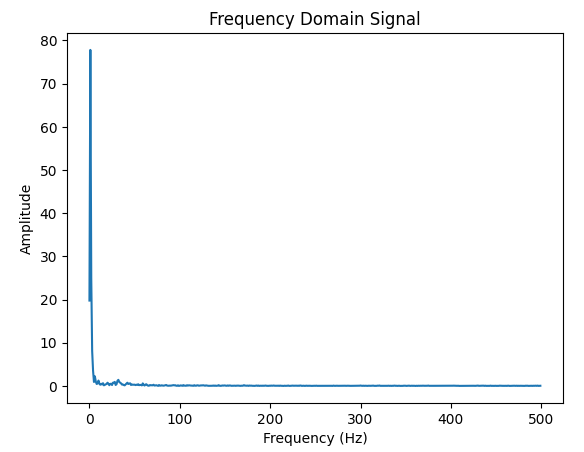
To evalute the accelerometer’s accuracy, I measured the output of the pitch and roll functions where outputs of -90, 0, and 90 degrees were expected, with results displayed in the graphs below. Based on this data, the accelerometer seems to calculate the pitch and roll at these extreme values pretty accurately. I had very small mean error of <1 degree, so there was little need for offset adjustment, likely due to the low-pass filter already in the IMU. There was notably much smaller amounts of noise for roll than pitch shown on the Fast Fourier transform plots.

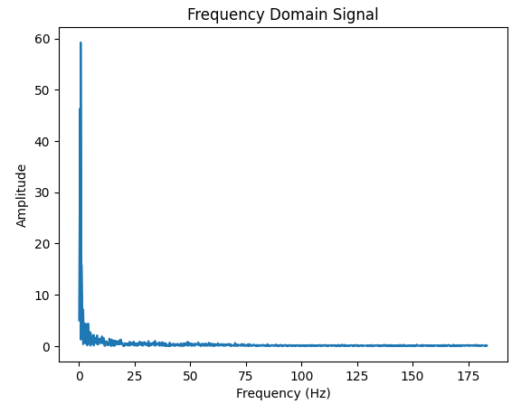
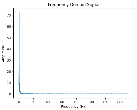
A good choice for cutoff frequency might be around 5 Hz, as there doesn’t seem to be useful data beyond this point for either axis. Implementing a simple low-pass filter using this cutoff frequency, I had a sampling frequency of about 350, so my alpha-value for my chosen cutoff frequency came to about 0.994. There were minor changes in pitch readings, and almost no changes in the roll measurements, which already had little noise.

Gyroscope

For the gyroscope data, I implemented the differential equation shown below in the subsequent code snippet:

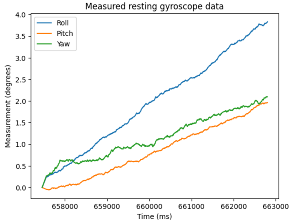
I first compared the resting measurements with no IMU movement. The gyroscope data had significantly less measurement noise, but since the roll and pitch were continuously incremented by their previous values while no movement occurred, they had substantial drift.

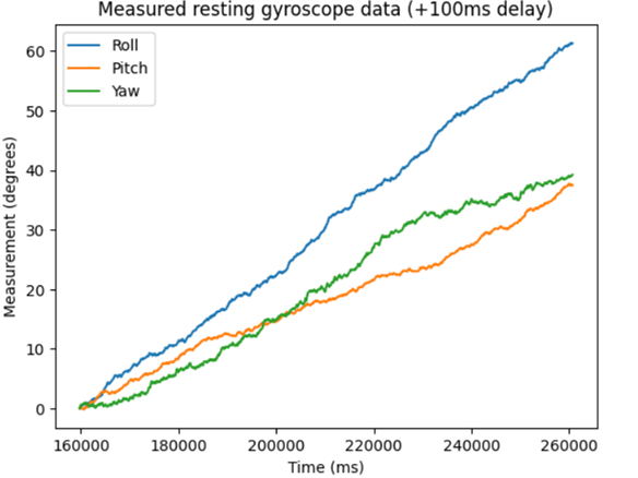
Delaying the sample frequency by ~100ms seemed to lower variance further to an extent, as this data was generally more linear.

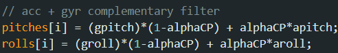
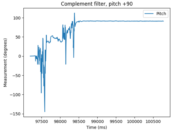
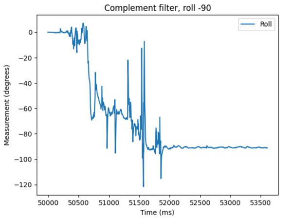
To counteract the drift, I implemented a complementary filter to combine the gyroscope and filtered accelerometer data. I retained the same low-pass parameter of 0.935, and eventually settled on a parameter of 0.4 for the complementary filter based on performance during long critical points in resting performance.

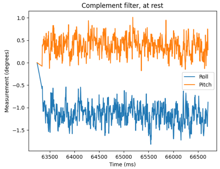
Compared to the previous methods, this combined the solid baseline of the accelerometer accuracy with the gyroscope precision while minimizing drift.

For demonstration, I took measurements at rest, at +90 pitch, and at -90 roll. My movements were rough, but steady behavior when held at each point was very consistent. However, at rest, I did notice an offset of around 0.5-1 degree for both roll and pitch. Pitch data was consistent with earlier, but roll data was a bit farther from the true angle than the raw accelerometer data on average.

Sample Data

I used the second approach from last lab to collect and store all the data in global arrays before sending it to my laptop via Bluetooth. After removing unnecessary computations, the fastest collection I measured was around 350 datapoints collected per second. It looks like my main loop outruns the IMU data updates, as my main delay was in accounting for that update speed.

A major contributor is that I was only measuring one dimension at a time for the accelerometer. I maintained 2 global 1000-element arrays for time and sensor data, and the Artemis had more than enough space with 384kB to store 8,000 bytes, plus three more global floats used for updating variables, for a total of 8,012 bytes.

For the gyroscope, I recorded everything at once, but maintained separate arrays for no particular reason. I think it would make more sense to store everything in one big array because keeping the entire array stored in one location avoids minor slow-downs from multiple searches for arrays that may be stored in multiple locations. Additionally, as these attributes would generally be accessed all at once for general locomotive purposes, it would be convenient for the data to be in the sam place.

For the data type, floats made the most sense as accuracy of data is important in state estimation, and small error can propagate to large miscalculations depending on control setting.

The accelerometer data, as well as most of the gyroscope data, was collected with a large sample size of 1000. Particularly, the gyroscope data before applying the complementary filter clearly demonstrates capturing for at least 5 seconds without the sampling rate delay, and for at least 10 seconds with the delay.

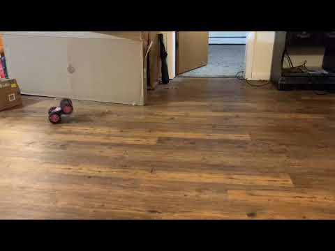
Record a Stunt

I tried out the RC car to finish out the lab. It was very difficult to control at first as it accelerated very quickly to full speed, which was convenient for long drives up and down the hallway, but not so much for the precision needed for tricks, especially with the basic controller sensitivity.

I was able to get a spinning wheelie, but I was unfortunately not able to reproduce it on camera. Here’s a failed attempt: