fast-robots

Lab 6

The purpose of this lab is to explore PID control again with sensor data to control the robot’s orientation.

Setup

Aside from a minor bug fix, I made no other changes to my strategy of sending/receiving messages over BlueTooth. I still use the same strategy as before:

A command from my laptop is sent to my robot containing the test PID values and a target value. I also added “max speed” and “max time” parameters to limit movement and execution time for debugging.
The robot executes a short test of PID sensor control using these values, recording sensor data during execution.
That data is then sent back to my laptop and processed in Python for data analysis.

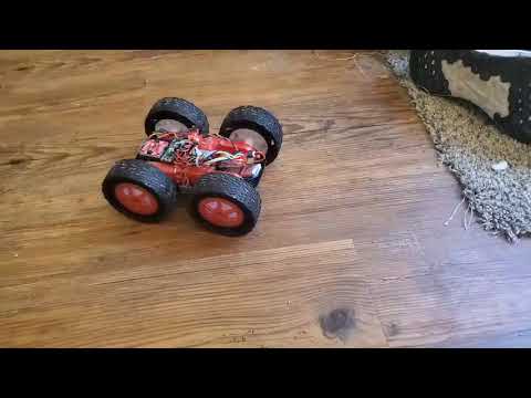
Limiting the speed was especially important as I noticed a minor hardware issue while working through this lab. The QWIIC port on my Arduino board is somewhat unstable and would disconnect when I turned too quickly.

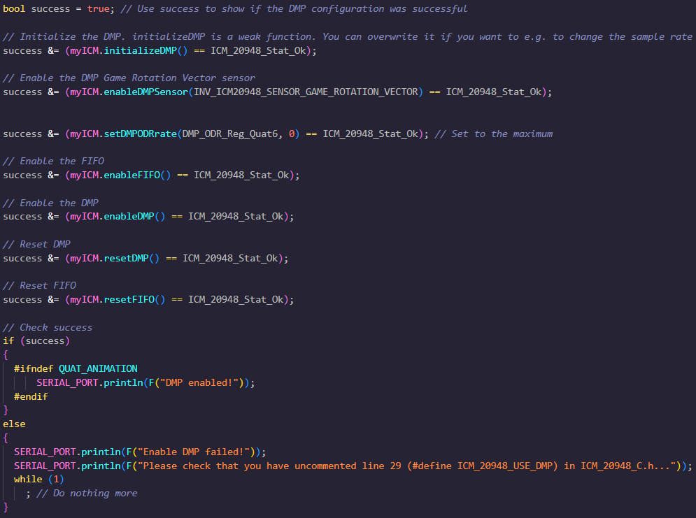
I also made some adjustments to my sensor data collection; namely, to reduce yaw drift, I enabled the digital motion processor (DMP) on the Arduino board and used it to combine gyroscope and accelerometer data from the IMU. After following the tutorial on the course website, I used some code from Example7 in the IMU example files to incorporate this in my robot code.

Particularly, I borrowed the following setup code:

setup code

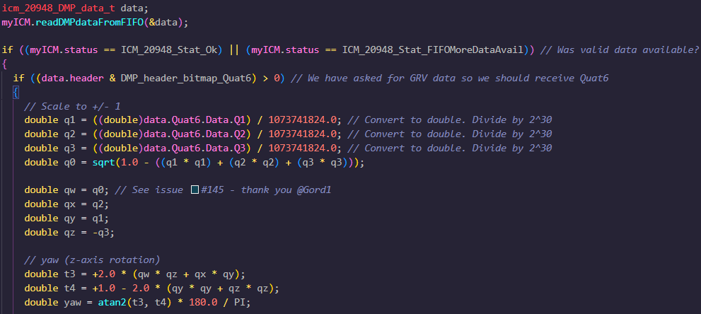
As well as this code for the data access and processing loop, omitting extraneous calculations:

loop code

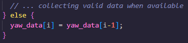
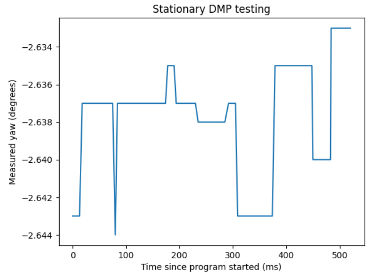
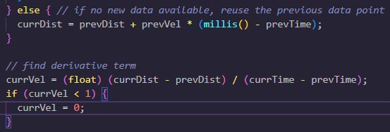
I also decided to use an extrapolative sampling method by reusing the previous yaw value when a new DMP datapoint was not available:

else branch

Judging against my sensor data from Lab 2, I looked at yaw measurements under various movement patterns. using the DMP seemed to stabilize the sensor data considerably. There admittedly wasn’t much variance before, but there seems to be even less deviation now.

dmp stationary test

Orientation Control

Using a strategy similar to Lab 5, I wrote a modified PID motor controller for robot orientation adjustments. Aside from the aforementioned, the only other changes were to change the sensor in use and swap car movement to rotation in place.

As described earlier, I used an extrapolation approach from Lab 5 and approximated new orientation values based on previous values whenever a new DMP reading was not yet available. Based on my sensor data, I could collect a full sample of ~500 data points in around 1900 milliseconds, which is slightly slower but comparable to the previous lab.

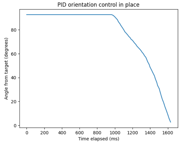
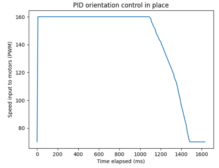
I started out using only a positional argument. For simple testing, I set up something similar to the previous lab. I put in a target value of a 90 degree rotation and started with a K_P value of 3 and a max speed of 200, which overshot its target pretty hard. I ended up reducing the K_P value to 2 and the speed to 180, which ended up being very effective. As shown below, the robot took a moment to get started with its rotation, but after it started moving it reached its destination very quickly. The PWM input to the motors followed expected behavior. My minimum speed based on lab 4 was 120 PWM, and after the car reached its target angle, no further inputs were calculated, which is why the speed graph never reaches 0 despite a successful test.

position data

speed data

Using only the P component seemed to be very effective, so I left things at that for now, but the implementation for I and D were left in the code for possible later development.

Applying the same logic, I wrote a loop that repeatedly checks the car’s orientation in live time and makes the necessary adjustments. This new command performs the following tasks:

The starting position/yaw is initialized outside of the while-loop.
At the start of every iteration, it gets a new yaw reading from the DMp if available, or reuses the previous value otherwise.
If the new value is far from the starting position, appropriate PWM values are sent to the motors until the car corrects its orientation, at which point it brakes.

I also made some small adjustments. I added a high-pass filter to the derivative to ignore small derivative values. Even though my derivative term went unused here, it was still used for data interpolation, so this was to make sure small derivative values would not result in “jittering” when interpolating new yaw values.

interpolate adjustment

In the future, I would like to make this more easily integrable with other code by rewriting this using a handler in the main Arduino loop that’s only called whenever the yaw value is changed.

Here I demonstrate my finished product: