fast-robots

Lab 7

The objective of this lab is to implement a Kalman filter algorithm to improve performance for Lab 5’s task of approaching a particular distance from a wall (1 meter) as quickly as possible from various distances (2-4 m) by refining distance data from the front-facing Time-of-Flight (ToF) sensor.

Setup

Aside from rewriting some old functions to use less data and save space, I have made no meaningful changes to my robot, or regarding sending/receiving messages via BLE between my laptop and my car robot, since the previous lab.

Estimating drag and momentum

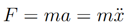
Following the derivation from lecture, Newton’s second law of motion states:

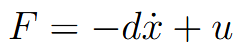
Additionally, the linear force acting on the car in terms of linear drag force d and motor input u:

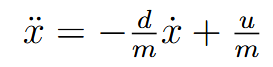
Using these, we can describe the dynamics of the robot car system as:

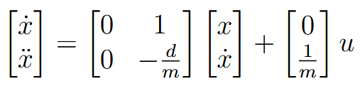
If we represent the system in state space notation in terms of position x and change in state x-dot:

Then we can rewrite the dynamics statement in the form Ax + Bu:

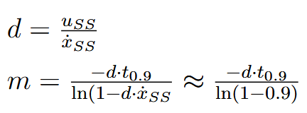
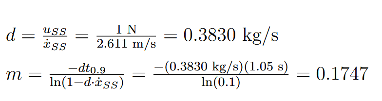
Again drawing from lecture, we can estimate the drag and mass using the following equations in terms of steady-state speed, steady-state input, and 90% rise time:

To find those values, I wrote a program that measures motor PWM inputs and ToF distance measurements over time. During data collection, the car starts at a distance of ~4000 mm and is set to run at a wall at a constant motor input. I used a 200 PWM input to be consistent with Lab 5 conditions. To avoid damaging the car, I put up a foam sheet and added active breaking in the code when the car gets within ~1 meter of the wall. Below is a brief video demonstration:

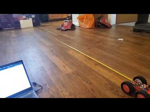
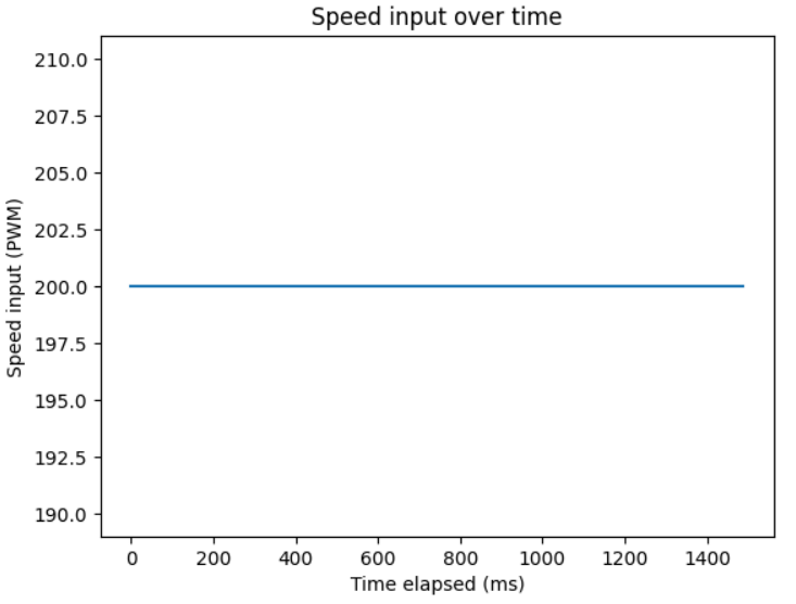
As shown in the video, the active braking and foam were very effective in minimizing damage to my car. Below is my collected motor PWM input and measured TOF distance data:

I then converted distance measurements to velocity values in Python by taking differences between adjacent data points at each measurement time. Below is the aforementioned Python code and the resulting graph, annotated to highlight target values:

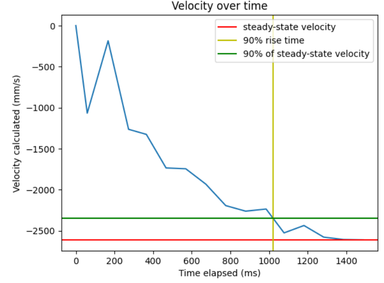
Based on this data, my steady-state velocity seems to be approximately 2.610 meters per second. At 90% rise time around ~1.05 seconds, the speed was around 2.349 meters per second. It follows that the drag and momentum terms are found as follows:

Initializing Kalman Filter

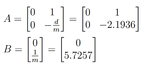
Given previously calculated values and simplifying, I find the following A and B matrices:

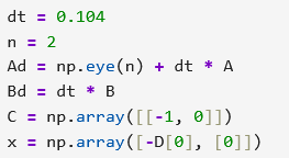
Based on my experimental data from the previous section, I sampled 100 data points in 10.412 seconds, so my sampling rate is 0.104 second. The dimension of the state space is clearly 2, so I discretize these matrices in Python. Next, I initialize state vector x based on the first measured ToF value, which was 4098 mm in this case, and define observation matrix C by following the recommendation from the lab handout and using a matrix of [-1 0]^T measuring negative distance from the wall. All of these operations are compiled below. (Note that my experimental observations are stored in an array called [D] instead of [tof].)

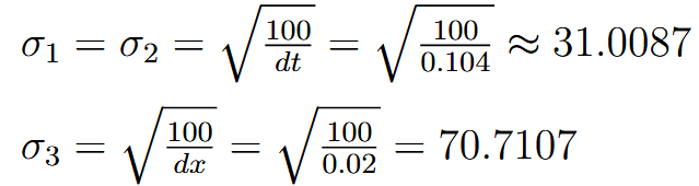
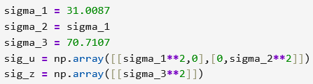
Finally, following from lecture, I select initial process noise and sensor noise covariance matrices using equations from lecture. (Here, I select dx = 20 mm = 0.02 m based on the sensor error data from the ToF sensor data sheet in long-range mode in worst-case lighting.)

Then I substitute these values appropriately into process noise and sensor noise covariance matrices under assumption of uncorrelated noise:

Implementation and testing of Kalman filter in Python

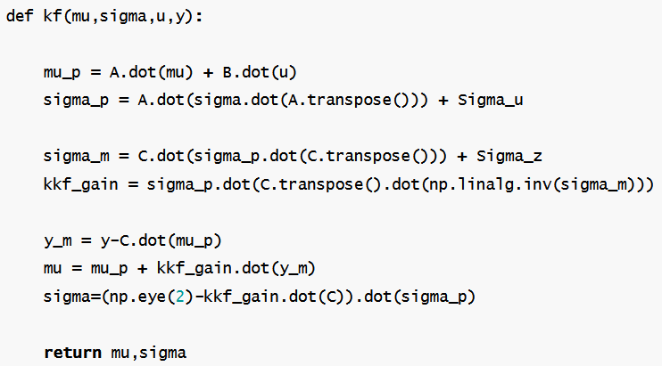
To finish a Python version of my Kalman filter for testing, I use the Kalman filter update implementation shown in lecture:

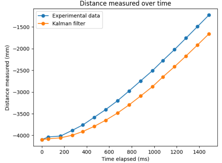
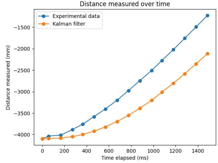
Below are the Kalman filter results plotted against my experimental data. Although the shape seems appropriate in terms of smoothness and relative form compared to experimental data, the Kalman filter results were a considerable overestimate of the true distance from the wall. (Note that all the values in the graph are flipped to be consistent with our state representation, so this is an overestimate of the absolute value distance from the wall.)

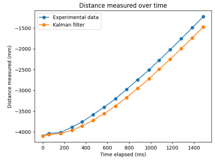
This means that my covariance matrix estimates must be improved. I tried increasing the dx value, putting more faith in my sensor measurements as this would decrease [sigma_3], and this brought the graph closer and closer to the experimental data. Below I demonstrate with a value of 0.05:

Similarly, when I decreased dx and and my faith in my sensor measurements, the filter values strayed further from the experimental data and relied more on the model. Below I demonstrate with a value of 0.005:

Implementation and testing of Kalman filter on Artemis

I stuck with a dx value of 0.02 for this part. I wrote a new robot command to run the Kalman filter procedure onboard the Artemis.